Basics of Statistics in Physical Education – BPEd ( Semester IV )

Table of Contents

Unit 1:- Introduction to Statistics

Q 1. Definition of Statistics

a) Introduction To Statistics

In Physical Education and Sports, we deal with scores, timings, distances, fitness levels, and performance records. To understand and analyze these numbers properly, we use Statistics.

👉 Statistics helps us collect, organize, analyze, and interpret data so that we can make correct decisions.

DEFINITION OF STATISTICS

Simple Definition: Statistics is the science of collecting, organizing, analyzing, and interpreting numerical data.

Classical Definitions (Easy Language):

✅ i) According to Croxton and Cowden: Statistics is the science that deals with the collection, analysis, and interpretation of numerical data.

✅ ii) According to Bowley: Statistics are numerical statements of facts placed in relation to each other.

b) Explanation In Simple Words

Statistics means:

Collecting data → fitness scores, timings
Organizing data → tables, charts
Analyzing data → average, comparison
Interpreting data → drawing conclusions

Examples Related To Physical Education

Example 1: Fitness Test

Collect push-up scores of students
Find the average (mean)
Compare boys and girls
👉 This whole process is Statistics

Example 2: Sports Performance

Record 100 m running times
Arrange them in a table
Identify the best and average performers
👉 Use of Statistics

Example 3: Training Program

Measure endurance before and after training
Compare results
Decide whether training was effective
👉 Statistical analysis

c) Why Statistics Is Important in Physical Education

Helps in the evaluation of performance
Useful in player selection
Assists in planning training programs
Supports scientific research
Helps in decision-making

STATISTICS IN ONE SIMPLE LINE

Statistics helps Physical Education teachers and coaches understand performance data and take scientific decisions.

d) Connection With Introduction To Statistics

Introduction Point	Explanation
What is Statistics?	Study of numerical data
Why Statistics?	To understand performance
Use in PE	Fitness, sports, training
Outcome	Better decisions

CONCLUSION: Statistics is the backbone of Physical Education research and performance evaluation, turning raw numbers into meaningful information.

Q > Need and importance of Statistics in Physical Education and Sports.

Statistics In Physical Education & Sports

Statistics is the science of collecting, organizing, analyzing, and interpreting data related to physical fitness, sports performance, health, and training.

a) 20 POINTS OF NEED OF STATISTICS

(Why Statistics is needed in Physical Education & Sports)

✅ i) Systematic Data Collection

Statistics help to collect data properly and scientifically.
In Physical Education, data like height, weight, timing, and scores are collected.
Without statistics, data becomes disorganized.
Example: Recording 100m race timings of students.

✅ ii) Organization of Large Data

Sports data is usually large in number.
Statistics help to arrange data in tables and charts.
This makes data easy to understand.
Example: Organizing fitness test results of a whole class.

✅ iii) Simplification of Data

Statistics converts complex data into a simple form.
Mean, graphs, and charts make understanding easy.
Students learn faster through simplified data.
Example: Finding the average weight of students.

✅ iv) Comparison of Performance

Statistics help to compare the performance of players or students.
Comparison shows improvement or decline.
It supports fair judgment.
Example: Comparing the jump distance of two athletes.

✅ v) Evaluation of Physical Fitness

Fitness components are measured using statistical tools.
It shows fitness level clearly.
Helps in identifying fit and unfit students.
Example: Fitness test score analysis.

✅ vi) Measurement of Training Effect

Statistics check the effectiveness of training programs.
Pre-test and post-test data are compared.
Improvement is measured scientifically.
Example: Speed improvement after training.

✅ vii) Selection of Players

Statistics hhelpin selecting players based on performance.
Selection becomes fair and unbiased.
Merit gets priority.
Example: Team selection based on timing.

✅ viii) Game Performance Analysis

Statistics analyze game performance.
Strengths and weaknesses are identified.
It helps in strategy making.
Example: Number of goals scored and missed.

✅ ix) Prediction of Performance

Statistics help in predicting future performance.
Records are used for analysis.
Helps in planning training.
Example: Predicting medal chances.

✅ x) Improvement in Teaching

Teachers use statistics to check teaching effectiveness.
Student performance reflects teaching quality.
Teaching methods can be improved.
Example: Test result comparison.

✅ xi) Research Work

Statistics is essential for research in Physical Education.
It helps in analysis and conclusion.
Research becomes scientific.
Example: Research on yoga and flexibility.

✅ xii) Control of Training Load

Statistics help control over-training and under-training.
Training load can be adjusted.
Injuries are reduced.
Example: Monitoring heart rate.

✅ xiii) Evaluation of Competition Results

Statistics help in ranking players and teams.
Results become clear and fair.
Ensures transparency.
Example: Sports meet results.

✅ xiv) Identification of Weak Areas

Statistics highlight weak areas of performance.
Focused training can be given.
Overall performance improves.
Example: Low stamina shown in the endurance test.

✅ xv) Maintenance of Records

Statistics help maintain sports records.
Data is stored for future use.
Helps with reference and planning.
Example: Annual sports records.

✅ xvi) Decision Making

Statistics support correct decision-making.
Decisions are based on facts.
Reduces guesswork.
Example: Choosing a team captain.

✅ xvii) Motivation of Students

Statistics show progress clearly.
Students feel motivated to improve.
Encourages healthy competition.
Example: Fitness improvement chart.

✅ xviii) Planning of Sports Programs

Statistics help in proper sports planning.
Time and resources are used effectively.
Programs become successful.
Example: Planning a training schedule.

✅ xix) Evaluation of Health Status

Statistics help in checking health conditions
BMI, pulse rate, etc., are analyzed.
Early health issues are detected.
Example: BMI calculation.

✅ xx) Sports AdministrationStatistics help in sports management.

It supports planning and budgeting.
Administration becomes effective.
Example: Participation data analysis.

b) 20 POINTS OF IMPORTANCE OF STATISTICS

(Why Statistics is important in Physical Education & Sports)

✅ i) Scientific Foundation

Statistics give a scientific base to Physical Education.
All activities are measured logically.
Results become reliable.
Example: Fitness evaluation.

✅ ii) Accuracy in Measurement

Statistics ensure accurate measurement.
Errors are minimized.
Results are trustworthy.
Example: Accurate timing system.

✅ iii) Objective Evaluation

Statistics removes personal bias.
Evaluation becomes fair.
Students trust the results.
Example: Merit-based selection.

✅ iv) Performance Improvement

Statistics help monitor improvement.
Weaknesses are identified.
Performance improves gradually.
Example: Progress report of an athlete.

✅ v) Effective Coaching

Coaches plan training scientifically.
Individual training is possible.
Performance level increases.
Example: Strength training plan.

✅ vi) Player Development

Statistics help in long-term player development.
Progress is tracked regularly.
Career planning becomes easy.
Example: Age-wise performance chart.

✅ vii) Injury Prevention

Statistics help prevent sports injuries.
Training load is monitored.
Athletes remain safe.
Example: Monitoring workload.

✅ viii) Fair Selection Process

Statistics ensure fair player selection.
Talent is recognized.
Bias is reduced.
Example: Selection trials data.

✅ ix) Improvement of Competition Standard

Statistics improves quality of competition.
Ranking and scoring are clear.
Sports become professional.
Example: League table.

✅ x) Effective Evaluation System

Evaluation becomes clear and systematic.
Feedback improves performance.
Learning becomes better.
Example: Fitness scorecard.

✅ xi) Helpful in Research

Statistics is the backbone of sports research.
Results become valid.
New knowledge is developed.
Example: Research on endurance training.

✅ xii) Planning & Policy Making

Statistics help in sports planning and policies.
Decisions are data-based.
Resources are used properly.
Example: National sports schemes.

✅ xiii) Motivation & Goal Setting

Statistics motivate athletes.
Clear goals are set.
Progress is measurable.
Example: Target time achievement.

✅ xiv) Talent Identification

Statistics help identify sports talent early.
Young athletes are trained properly.
Future champions are developed.
Example: Junior athlete performance.

✅ xv) Game Strategy Development

Statistics help in making game strategies.
Opponent analysis becomes easy.
Winning chances increase.
Example: Match statistics.

✅ xvi) Analysis of Records

Statistics help analyze sports records.
New records are set.
Performance standards rise.
Example: Olympic records.

✅ xvii) Health Awareness

Statistics increase health awareness.
Fitness levels are known.
Prevention is better than a cure.
Example: Health survey data.

✅ xviii) Evaluation of Sports Programs

Statistics evaluate sports programs.
Success and failure are identified.
Improvements are made.
Example: School fitness program.

✅ xix) Professional Growth of Teachers

Statistics improves professional skills of PE teachers.
Research skills increase.
Teaching quality improves.
Example: Action research.

✅ xx) National Sports Development

Statistics help in national sports development.
Performance data guides planning.
The country’ssports level improves.
Example: Olympic medal analysis.

c) Comparative Summary Table

(Need vs Importance of Statistics in Physical Education & Sports)

S.No	Need for Statistics	Importance of Statistics
1	Data collection	Scientific foundation
2	Data organization	Accurate measurement
3	Data simplification	Objective evaluation
4	Performance comparison	Performance improvement
5	Fitness evaluation	Effective coaching
6	Training evaluation	Player development
7	Player selection	Injury prevention
8	Game analysis	Fair selection
9	Performance prediction	Better competition
10	Teaching improvement	Effective evaluation
11	Research work	Research support
12	Training load control	Planning & policy
13	Result evaluation	Motivation
14	Weakness identification	Talent identification
15	Record maintenance	Strategy development
16	Decision making	Record analysis
17	Motivation	Health awareness
18	Sports planning	Program evaluation
19	Health evaluation	Professional growth
20	Sports administration	National sports development

Q > Scope of Statistics in Physical Education & Sports

a) 20 Points Of Scope Of Statistics

✅ i) Measurement of Physical Fitness

Statistics is used to measure physical fitness components.
Strength, speed, endurance, and flexibility are evaluated.
Results are recorded and compared.
Example: Fitness test scores of students.

✅ ii) Evaluation of Sports Performance

Statistics help to evaluate individual and team performance.
Performance improvement or decline is identified.
Helps in giving proper feedback.
Example: Match performance statistics.

✅ iii) Selection of Players

Statistics are used in the fair selection of players.
Performance data is analyzed.
The best performers are selected.
Example: Selecting sprinters based on timing.

✅ iv) Talent Identification

Statistics help identify sports talent at an early age.
Physical and skill tests are analyzed.
Future champions are developed.
Example: Junior athlete performance analysis.

✅ v) Training Program Planning

Statistics help plan effective training programs.
Training load and intensity are decided scientifically.
Improves performance safely.
Example: Weekly training schedule based on data.

✅ vi) Evaluation of Training Effect

Statistics checks whether the training is effective or not.
Pre-test and post-test results are compared.
Training can be modified.
Example: Speed improvement after training.

✅ vii) Game Strategy Development

Statistics help in planning game strategies.
Opponent strengths and weaknesses are studied.
Winning chances increase.
Example: Match analysis in cricket.

✅ viii) Research in Physical Education

Statistics is essential for research work.
It helps in data analysis and conclusion.
Research becomes scientific.
Example: Research on yoga and flexibility.

✅ ix) Sports Psychology

Statistics help study psychological factors.
Motivation, anxiety, and confidence are measured.
Improves mental preparation.
Example: Anxiety level survey before competition.

✅ x) Sports Medicine & Injury Management

Statistics help in injury analysis and prevention.
Injury patterns are studied.
Athlete safety improves.
Example: Injury rate analysis in football.

✅ xi) Health Assessment

Statistics help in evaluating health status.
BMI, heart rate, and blood pressure are analyzed.
Health risks are identified early.
Example: BMI calculation of students.

✅ xii) Curriculum Planning

Statistics help in planning the E curriculum.
Student performance data guides planning.
Curriculum becomes effective.
Example: Improving syllabus based on results.

✅ xiii) Evaluation of Teaching Methods

Statistics help evaluate teaching effectiveness.
Student results reflect teaching quality.
Methods can be improved.
Example: Test score comparison.

✅ xiv) Sports Administration

Statistics help in sports management.
Planning, budgeting, and organization become easy.
Administration improves.
Example: Participation data analysis.

✅ xvi) Conduct of Sports Competitions

Statistics help organize competitions.
Scoring, ranking, and results are managed.
Fair competition is ensured.
Example: Points table in tournaments.

✅ xvi) Maintenance of Sports Records

Statistics help maintain sports records.
Past performances are stored safely.
Useful for future reference.
Example: School sports achievement records.

✅ xvii) Performance Comparison

Statistics allow comparison between players and teams.
Strengths and weaknesses are identified.
Better decisions are taken.
Example: Comparing two athletes’ timings.

✅ xviii) Policy Making in Sports

Statistics support sports policy decisions.
Data helps in planning programs.
Development becomes systematic.
Example: Government sports schemes.

✅ xix) Motivation & Goal Setting

Statistics motivate athletes.
Progress can be seen clearly.
Goal setting becomes easy.
Example: Target improvement chart.

✅ xx) National Sports Development

Statistics help in national sports planning.
Performance data guides improvement.
Sports standards rise.
Example: Olympic performance analysis.

b) SUMMARY TABLE WITH SHORT NOTES

Scope of Statistics in Physical Education & Sports

S.No	Scope Area	Short Note
1	Physical fitness	Measures fitness components
2	Performance evaluation	Assesses performance
3	Player selection	Fair selection
4	Talent identification	Finds future talent
5	Training planning	Scientific training
6	Training evaluation	Checks effectiveness
7	Game strategy	Improves tactics
8	Research	Scientific studies
9	Sports psychology	Mental assessment
10	Sports medicine	Injury analysis
11	Health assessment	Health evaluation
12	Curriculum planning	Effective syllabus
13	Teaching evaluation	Improves teaching
14	Sports administration	Better management
15	Competitions	Fair results
16	Record maintenance	Preserves data
17	Performance comparison	Better decisions
18	Policy making	Sports development
19	Motivation	Goal setting
20	National sports	International success

EXAM TIP

Scope = Area of application
Write definition + 5–6 points for short answers.
Use examples to score a full mark

Q > Classification of Statistics

Classification Of Statistics In Physical Education & Sports

Statistics is divided into different types based on the kind of data, methods, and usage. Understanding classification helps teachers, coaches, and researchers to analyze data correctly.

a) Classification Of Statistics

Statistics can be mainly classified into two types:

✅ i) Descriptive Statistics

Descriptive statistics summarize and describe data.
It tells us “what happened” without making predictions.
Tools include mean, median, mode, graphs, tables, and charts.
Example: Calculating the average speed of 50 sprinters in a school.

Key Uses:

Organizes data
Simplifies complex data
Compares performance

✅ ii) Inferential Statistics (Analytical Statistics)

Inferential statistics draws conclusions or predictions from sample data about a larger group.
It tells us “what may happen” or tests hypotheses.
Tools include t-tests, ANOVA, correlation, and regression.
Example: Studying the effect of 6 weeks of training on endurance in a sample of 20 students to predict results for the whole class.

Key Uses:

Prediction and forecasting
Testing relationships
Scientific research

Sub-Classification (Optional for Students)

Type	Examples in Physical Education
Descriptive	Mean, Mode, Median, Range, Graphs
Inferential	t-test, ANOVA, Correlation, Regression

b) Summary Table (Comparison)

Feature	Descriptive Statistics	Inferential Statistics
Meaning	Summarizes & describes data	Draws conclusions & predictions
Purpose	“What happened?”	“What may happen?”
Tools	Mean, Median, Mode, Charts, Tables	t-test, ANOVA, Correlation, Regression
Usage	Organizing & comparing performance	Research, prediction & hypothesis testing
Example	Average height of students	Effect of training on performance

CONCLUSION: Descriptive statistics tells us what has happened, while inferential statistics helps us predict or analyze future outcomes in Physical Education and Sports.

Q > Intervals: Raw Score, Continuous and Discrete Series, Class Distribution, Construction of frequency table

a) Intervals: Raw Score

Raw Score:

The actual value or observation recorded in a test or measurement.
It is unprocessed data collected directly from students or athletes.
Example in Physical Education:
- Time taken by a student to run 100m: 14.5 seconds
- Jump distance in long jump: 2.8 meters
Intervals:
- When we group raw scores into ranges, we call them class intervals.
- Example: If 100m sprint times are 12.0, 12.5, 13.0, … we can create intervals like 12–12.9 sec, 13–13.9 sec, etc.

Key point: Raw scores are individual observations; intervals are groups of scores.

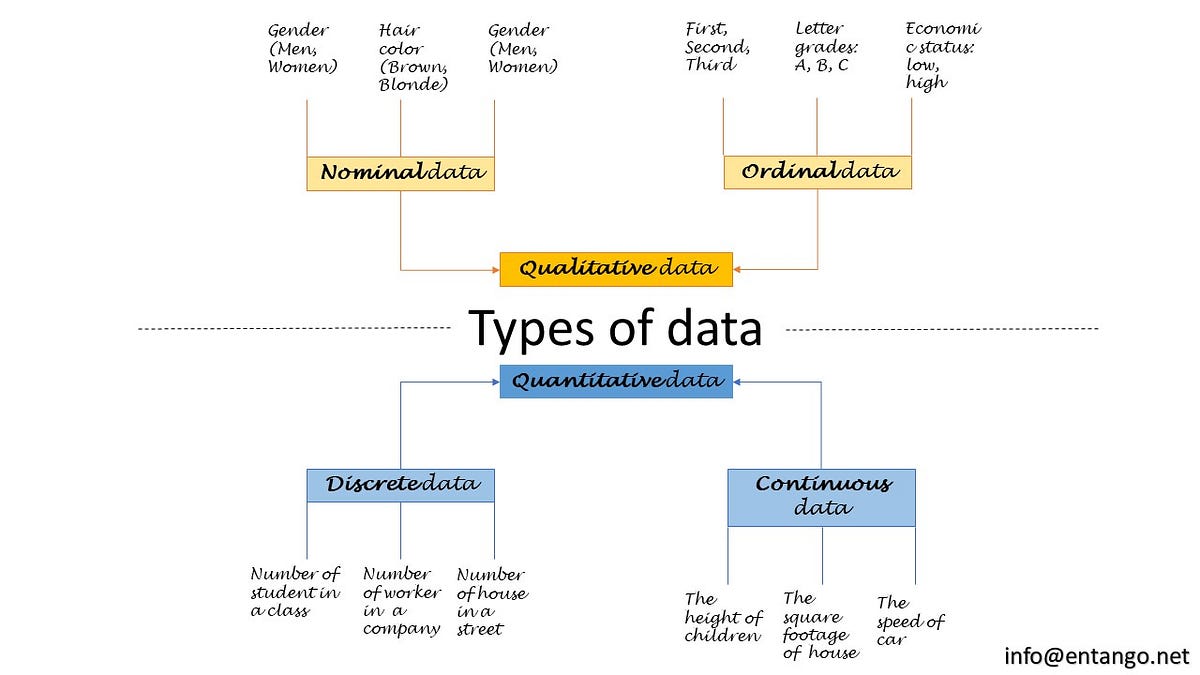
b) Continuous and Discrete Series

✅ i) Continuous Series:

Data that can take any value within a range.
Usually measured, not counted.
Example in Physical Education:
- Height of students: 165.2 cm, 170.5 cm, 172.0 cm
- Weight of athletes: 60.5 kg, 65.3 kg
Continuous data can be divided into intervals.

✅ ii) Discrete Series:

Data that can only take specific values.
Usually counted, not measured.
Example in Physical Education:
- Number of goals scored in a match: 0, 1, 2, 3
- Number of students participating in a tournament: 20, 25, 30
Discrete data cannot be divided into smaller parts.

c) Class Distribution

Definition:

When raw scores are grouped into classes/intervals, it forms a class distribution.
Shows how many observations fall in each interval.

Example:

Interval (Seconds)	Number of Students
12–12.9	3
13–13.9	5
14–14.9	7
15–15.9	5

Interpretation: Most students ran between 14–14.9 seconds.

Key point: Class distribution simplifies large data for easy understanding.

d) Construction of Frequency Table

Steps to Construct:

Collect Raw Scores – Example: 12.4, 13.1, 14.8, 15.2, 13.5…
Find Range – Range = Maximum score – Minimum score.
Decide Class Intervals – Group scores into intervals.
Tally Frequency – Count how many scores fall in each interval.
Create Table – Make a clear table showing intervals and frequency.

Example:

Interval (Sec)	Tally	Frequency
12–12.9
13–13.9
14–14.9
15–15.9

Observation: The frequency table shows how the data is distributed across intervals.

e) Summary Table

Concept	Meaning	Example in Physical Education
Raw Score	Original unprocessed data	100m sprint time = 14.5 sec
Interval	Grouping of raw scores	12–12.9 sec, 13–13.9 sec
Continuous Series	Data that can take any value	Height = 165.2, 170.5 cm
Discrete Series	Data that takes only specific values	Goals scored = 0,1,2,3
Class Distribution	Number of observations in each interval	12–12.9 sec = 3 students
Frequency Table	Table showing class intervals and frequency	Interval vs. number of students

🔹 Key Points to Remember:

Raw scores → original measurements
Intervals → grouped data
Continuous → measurable data (height, weight, time)
Discrete → countable data (goals, participants)
Frequency table & class distribution → simplifies data for analysis.

Unit 2 :- Basics of Statistical Analysis

Q > Graphical Presentation of Class Distribution: Histogram, Frequency Polygon, Frequency Curve. Cumulative Frequency Polygon, Ogive, Pie Diagram

GRAPHICAL PRESENTATION OF CLASS DISTRIBUTION (In Physical Education & Sports)

Graphical presentation means showing statistical data in the form of graphs or diagrams.
Graphs make data easy to understand, compare, and remember, especially for students of Physical Education.

a) Histogram

Meaning of Histogram

A Histogram is a graph used to represent continuous data.
It consists of rectangular bars with no gap between them.
Class intervals are shown on the X-axis, and frequency on the Y-axis.

Use of Histogram

Used when data is in class intervals.
Helps to see which class has the highest frequency.

Example (Physical Education)

Showing 100 m race timings of students:
- 12–13 sec, 13–14 sec, 14–15 sec, etc.
The tallest bar shows the interval where the maximum number of students fall.

b) Frequency Polygon

Meaning of Frequency Polygon

A Frequency Polygon is a line graph of a frequency distribution.
It is formed by joining the mid-points of class intervals with straight lines.

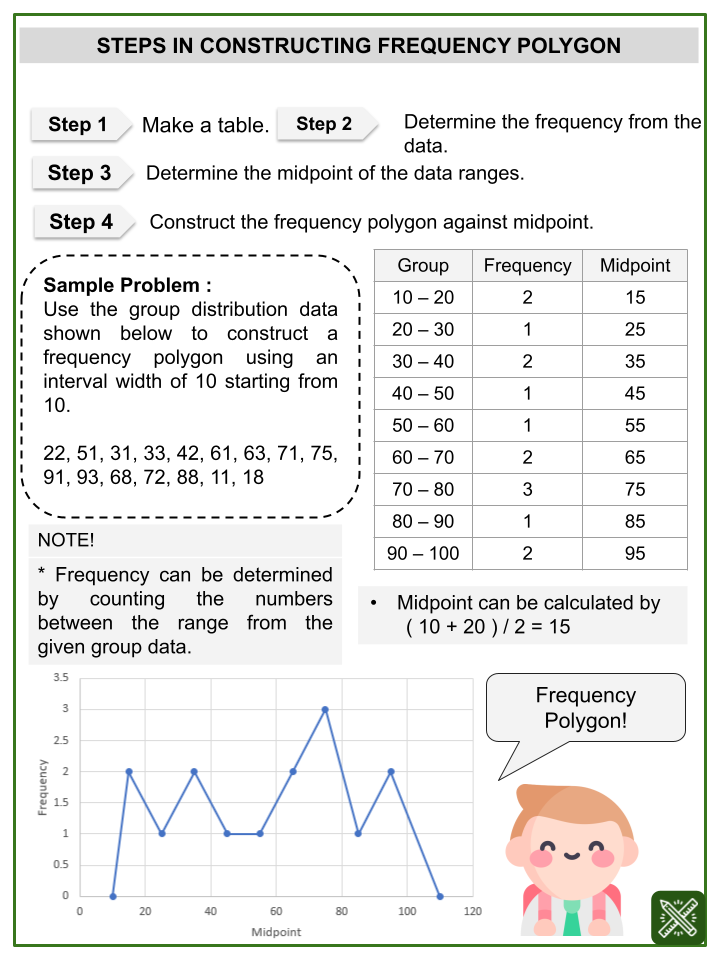
Use of Frequency Polygon

Used to compare two or more distributions.
Can be drawn with or without a histogram.

Example: Comparing boys’ and girls’ running performance in a 100 m race.

c) Frequency Curve

Meaning of Frequency Curve

A Frequency Curve is a smooth curved line drawn through the points of a frequency polygon.
It shows the overall pattern of distribution.

Use of Frequency Curve

Helps to study the nature of data (normal, skewed).
Used mainly in advanced analysis.

Example: Showing the general pattern of students’ fitness scores.

d) Cumulative Frequency Polygon

Meaning of Cumulative Frequency Polygon

A Cumulative Frequency Polygon is a graph that shows cumulative frequencies.
Frequencies are added class by class.

Use of Cumulative Frequency Polygon

Helps to find median, quartiles, and percentiles.
Shows how data accumulates.

Example: Total number of students scoring below a certain fitness score.

e) Ogive

Meaning of Ogive

An Ogive is a graph of cumulative frequency.
There are two types:
- Less-than Ogive
- More-than Ogive

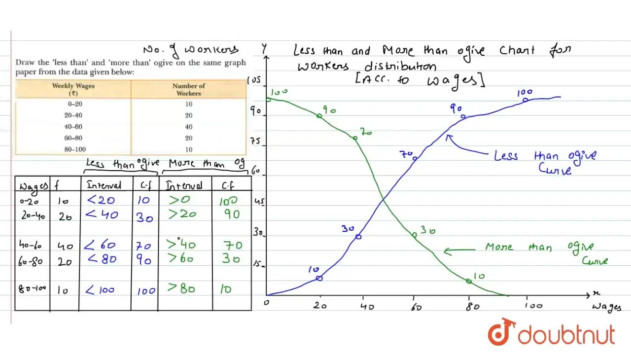
Use of Ogive

Used to find the median and quartiles graphically.
The intersection point of both ogives gives the median.

Example: Finding the median score of students in a fitness test.

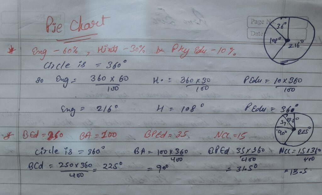
f) Pie Diagram

Meaning of Pie Diagram

A Pie Diagram is a circular graph.
The whole circle represents 100% of the data.
Each part shows the proportion of data.

Use of Pie Diagram

Used for percentage and ratio comparison.
Very attractive and easy to understand.

Example

Showing the distribution of students in different sports:
- Football – 40%,
- Cricket – 30%,
- Athletics – 20%,
- Others – 10%.

g) SUMMARY TABLE

Graph Type	Used For	Type of Data	Example in Physical Education
Histogram	Show class frequency	Continuous	100 m race timings
Frequency Polygon	Compare distributions	Continuous	Boys vs Girls performance
Frequency Curve	Show data pattern	Continuous	Fitness score trend
Cumulative Frequency Polygon	Accumulated data	Continuous	Scores below a value
Ogive	Median & quartiles	Continuous	Median fitness score
Pie Diagram	Percentage comparison	Any (Categorical)	Sports participation

🔑 Key Points to Remember (Exam Tip)

Histogram → Bars without gaps
Frequency Polygon → Straight lines
Frequency Curve → Smooth curve
Ogive → Cumulative frequency
Pie Diagram → Percentage distribution

Q > Measures of Central Tendency: Mean, Median, and Mode-Meaning, Definition, Importance, Advantages, Disadvantages, and Calculation from Group and Ungrouped data

MEASURES OF CENTRAL TENDENCY (In Physical Education & Sports)

Measures of Central Tendency are statistical methods used to find one central or average value that represents the whole data. Its help us find one central value that represents the overall performance of students or athletes.

a) MEAN (Arithmetic Mean)

Meaning

Mean is the average value of all observations.
It is calculated by adding all values and dividing by the total number of observations.
Mean is the most commonly used measure.

🔹 Calculation of Mean

✅ i) Mean from Ungrouped Data

Example (100 m race times in seconds):
- 12, 14, 13, 15, 16
Mean = (12 + 14 + 13 + 15 + 16) ÷ 5
- Mean = 14 seconds

✅ ii) Mean from Grouped Data

Class (sec)	f	Mid-value (x)	fx
12–14	2	13	26
14–16	3	15	45
16–18	1	17	17
Total	6		88

Mean = Σfx ÷ Σf = 88 ÷ 6 = 14.67 sec

Uses

Shows the overall performance level
Used in test evaluation and research

Limitation: The Mean is affected by very high or very low scores.

SNo	Importance (Mean)	Advantages (Mean)	Disadvantages (Mean)
1	Shows the overall performance level of a group	Easy to understand	Affected by extreme values
2	Commonly used in fitness and skill tests.	Easy to calculate	Not suitable for skewed data
3	Helps in comparison between groups	Uses all values	Cannot be used for qualitative data
4	Useful in sports research	Fixed and definite value	Sometimes misleading
5	Basis for many advanced statistics	Useful for further analysis	Difficult with open-ended classes
6	Helps teachers evaluate class performance	Most popular average	Requires all values
7	Useful for norms and standards	Good for large data	Not suitable when data is irregular
8	Helps in progress tracking	Represents whole data	May not represent typical value
9	Used in training evaluation	Suitable for comparison	Time-consuming for large data
10	Supports scientific decision-making	Useful in normal distributions	Not easy to calculate mentally

b) MEDIAN

Meaning

Median is the middle value of the data when arranged in ascending or descending order.
It divides the data into two equal parts.

🔹 Calculation of Median

✅ i) Median from Ungrouped Data

Example: 18, 20, 22, 24, 26
- Median = 22
If even values:
- 18, 20, 22, 24
- Median = (20 + 22) ÷ 2 = 21

✅ ii) Median from Grouped Data

Class	Frequency (f)	Cumulative Frequency
10–20	5	5
20–30	9	14
30–40	6	20

N = 20 → N/2 = 10
- Median class = 20–30
Median = l + (N/2–cf)÷f(N/2 – cf) ÷ f(N/2–cf)÷f × h
- = 20 + (10–5)÷9(10 – 5) ÷ 9(10–5

Uses

Useful when data has extreme values
Good for skewed data

Limitation: Does not use all values in the calculation.

SNo	Importance (Median)	Advantages (Median)	Disadvantages (Median)
1	Best for skewed data	Simple to calculate	Does not use all values
2	Not affected by extreme values	Not affected by extremes	Not suitable for further calculations
3	Useful for height and weight data	Useful for open-ended classes	Less accurate than the mean
4	Shows middle performance	Good for qualitative ranking	Requires data arrangement
5	Easy to understand	Easy to locate graphically	Cannot be algebraically treated
6	Helpful in uneven distributions	Suitable for skewed data	May not represent the whole data
7	Used in fitness evaluation	Stable value	Time-consuming for large data
8	Good for comparison	Clear middle position	Not useful in advanced statistics
9	Useful when the mean is misleading.	Useful in PE tests	Depends on the order of data
10	Represents a typical value	Requires fewer calculations	Limited analytical use

c) MODE

Meaning

Mode is the value that occurs most frequently in the data.
A dataset can have one mode, more than one mode, or no mode.

🔹 Calculation of Mode

✅ i) Mode from Ungrouped Data

Example: 12, 14, 14, 15, 16
Mode = 14

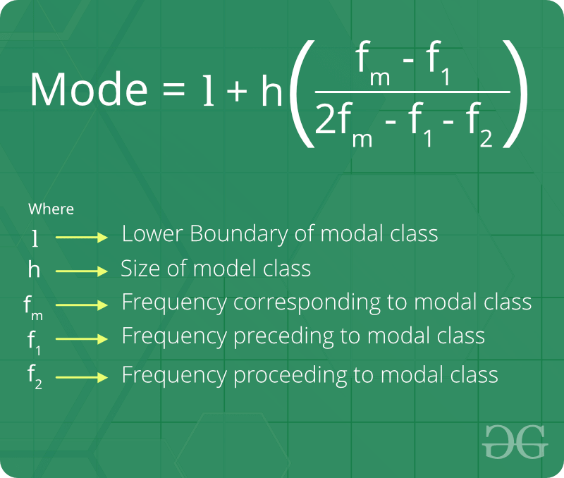
✅ ii) Mode from Grouped Data

Class	Frequency
10–20	6
20–30	12 ← Modal class
30–40	7

Mode = l + (f1–f0)÷(2f1–f0–f2)(f₁ – f₀) ÷ (2f₁ – f₀ – f₂)(f1–f0)÷(2f1–f0–f2) × h
= 20 + (12–6)÷(24–6–7)(12 – 6) ÷ (24 – 6 – 7)(12–6)÷(24–6–7) × 10
= 25.4

Uses

Easy to understand
Useful for categorical data

Limitation: Sometimes, no clear mode exists.

SNo	Importance (Mode)	Advantages (Mode)	Disadvantages (Mode)
1	Shows the most common performance	Very easy to find	May not exist
2	Useful in skill frequency analysis	No calculation needed	May have more than one value
3	Simple to understand	Not affected by extremes	Not stable
4	Useful for qualitative data	Useful for nominal data	Not based on all values.
5	Helps in grouping students	Can be found by inspection	Not suitable for further calculations
6	Not affected by extremes	Simple for students	Sometimes misleading
7	Used in sports participation data	Applicable to open classes	Not useful for small data
8	Indicates typical score	Shows popular value	Difficult in flat distributions
9	Useful for quick decisions	Useful in PE classes	Limited analytical value
10	Helps in basic comparisons	Time-saving	Not precise

d) SUMMARY TABLE

Measure	Meaning	Best Use	How to Find	Main Use	Main Advantage	Main Limitation	PE Example
Mean	Average value	Normal data	Sum ÷ Number	Overall performance	Uses all values	Affected by extremes	Avg race time
Median	Middle value	Skewed data	Arrange data	Skewed data	No extreme effect	Ignores some data	Middle jump
Mode	Most frequent value	Common score	Highest frequency	Common performance	Very simple	May not exist	Common score

🔑 Key Points to Remember

Mean → Arithmetic average
Median → Middle value
Mode → Most repeated value

Conclusion: Measures of central tendency help us understand the average performance level of students or athletes in Physical Education, teachers, and coaches.

Q > Measures of Variability: Meaning, importance, computing from group and ungroup data

MEASURES OF VARIABILITY (In Physical Education & Sports)

Meaning (Introduction)

Measures of Variability show how much the data values differ from each other or how spread out the data is around the average. While Measures of Central Tendency tell us the average, Variability tells us the consistency or uniformity of performance.

Example: Two teams may have the same average fitness score, but one team may be more consistent. Variability helps us identify this.

a) MEANING OF MEASURES OF VARIABILITY

Measures of Variability indicate the degree of dispersion or spread of scores in a data set.
They show whether performances are closely grouped or widely scattered.

Common Measures of Variability:

Range
Quartile Deviation (QD)
Mean Deviation (MD)
Standard Deviation (SD)

b) IMPORTANCE OF MEASURES OF VARIABILITY

Shows consistency of performance
Helps compare two groups with the same average
Indicates the reliability of data
Useful in player selection
Helps coaches in training planning
Identifies performance gaps
Useful in sports research
Shows the degree of individual differences
Helps in the evaluation of fitness tests
Supports scientific decision-making

c) COMPUTING MEASURES OF VARIABILITY

From Ungrouped and Grouped Data

✅ i) RANGE

Meaning: Range is the difference between the highest and lowest values.
Formula: Range = Highest value – Lowest value
Example:
- Ungrouped Data
  - Scores: 10, 12, 14, 16, 18
  - Range = 18 – 10 = 8
- Grouped Data: Take the upper limit of the highest class – lower limit of the lowest class. Example:
  - Classes: 10–20, 20–30, 30–40
  - Range = 40 – 10 = 30

✅ ii) QUARTILE DEVIATION (QD)

Meaning: Quartile Deviation shows the spread of the middle 50% of data.
Formula: QD = (Q₃ – Q₁) ÷ 2
Example:
- Ungrouped Data Example
  - Data: 10, 12, 14, 16, 18, 20
  - Q₁ = 12, Q₃ = 18
  - QD = (18 – 12) ÷ 2 = 3
- Grouped Data
  - Find Q₁ and Q₃ using the cumulative frequency table, then apply the formula.

✅ iii) MEAN DEVIATION (MD)

Meaning: Mean Deviation is the average of the absolute deviations from the mean or median.
Formula: MD = Σ|x – A| ÷ N
Example:
Ungrouped Data Example
- Data: 10, 12, 14
- Mean = 12
- MD = (|10–12| + |12–12| + |14–12|) ÷ 3
  - = (2 + 0 + 2) ÷ 3 = 1.33
Grouped Data
- MD = Σf|x – A| ÷ Σf

✅ iv) STANDARD DEVIATION (SD)

Meaning:
- Standard Deviation is the most important and accurate measure of variability.
- It shows how much values deviate from the mean.
Formula: SD = √(Σ(x – x̄)² ÷ N)
Example:
- Ungrouped Data Example
  - Data: 10, 12, 14
  - Mean = 12
  - SD = √[(4 + 0 + 4) ÷ 3]
  - SD = √(2.67) = 1.63
- Grouped Data
  - SD = √(Σf(x – x̄)² ÷ Σf)

d) SUMMARY TABLE

SNo	Measure	Meaning	Formula (Simple)	Use in PE
1	Range	Difference between the highest & the lowest	H – L	Quick comparison
2	Quartile Deviation	Spread of middle 50%	(Q₃–Q₁)/2	Consistency check
3	Mean Deviation	Avg deviation from mean	Σ\|x – A\| ÷ N	Performance varies widely
4	Standard Deviation	Best measure of spread	√Σ(x–x̄)²/N	Research & training

🔑 Key Exam Points

Central Tendency = Average
Variability = Spread / Consistency
Low variability = more consistent performance
SD is the most reliable measure.

Conclusion: Measures of Variability help Physical Education teachers and coaches understand the consistency and spread of performance, not just the average.

Q > Range, Standard deviation, Quartiles, Percentiles.

What are Measures of Variability?

Measures of Variability tell us how much the scores differ from each other.
They help us understand the spread, dispersion, or consistency of performance, not just the average.

Example: Two teams may have the same average running time, but one team may be more consistent. Variability shows this difference.

a) RANGE

Meaning: Range is the difference between the highest and lowest scores in a data set.
Formula: Range = Highest value – Lowest value
Example (Physical Education)
- 100 m running times (seconds):
- 12, 13, 14, 15, 16
- Range = 16 – 12 = 4 seconds
Importance
- Very easy to calculate
- Gives a quick idea about the spread
- Useful for rough comparison
Limitation
- Based only on two values
- Not very reliable

b) STANDARD DEVIATION (SD)

Meaning
- Standard Deviation shows how much scores differ from the average (mean).
- It is the most accurate and important measure of variability.
Interpretation
- Small SD → Scores are close to the mean (high consistency)
- Large SD → Scores are scattered (low consistency)
Simple Formula
- SD = √(Σ(x − x̄)² ÷ N)
Example (Simplified)
- Scores in vertical jump (cm):
- 40, 42, 44
- Mean = 42
- SD = √[(4 + 0 + 4) ÷ 3]
- SD ≈ 1.63
Importance in PE
- Used in sports research
- Helps in player selection
- Shows performance consistency

c) QUARTILES

Meaning
- Quartiles divide the data into four equal parts.
- They help understand the distribution of scores.
Types of Quartiles
- Q₁ (First Quartile) – 25% scores below
- Q₂ (Second Quartile / Median) – 50% scores below
- Q₃ (Third Quartile) – 75% scores below
Example
- Fitness scores:
- 10, 12, 14, 16, 18, 20
- Q₁ = 12
- Q₂ = 15
- Q₃ = 18
Use in Physical Education
- Shows the middle spread of performance
- Useful in ranking players

d) PERCENTILES

Meaning
- Percentiles divide the data into 100 equal parts.
- They show a person’s position in a group.
Common Percentiles
- P10 – Bottom 10%
- P50 – Median
- P90 – Top 10%
Example (Sports Test)
- If a student is at P80 in a fitness test,
- He/she performed better than 80% students.
Importance of Physical Education
- Used in fitness norms
- Helpful for talent identification
- Used in grading and evaluation

e) SUMMARY TABLE

Measure	Meaning	Key Formula	Use in Physical Education	Example
Range	Difference between the highest & the lowest	H − L	Quick spread check	16 − 12 = 4
Standard Deviation	Spread around the mean	√Σ(x−x̄)²/N	Consistency & research	SD = 1.63
Quartiles	Divide the data into 4 parts	Q₁, Q₂, Q₃	Ranking & distribution	Q₁=12
Percentiles	Divide the data into 100 parts	P10–P90	Norms & evaluation	P80 rank

Conclusion: Measures of Variability help Physical Education teachers and coaches understand how consistent or scattered performances are, beyond just the average.

Unit 3 :- The Normal Distribution & Correlation

Q > Introduction, probability of an event, Binomial distribution

a) INTRODUCTION TO PROBABILITY

Meaning

Probability means the chance or likelihood that an event will happen.
It tells us how likely or unlikely a result is.

Value of Probability

Probability always lies between 0 and 1
0 → Event will never happen
1 → Event will definitely happen

Example (Sports)

Chance of winning a match
Chance of scoring a goal
Chance of a player getting selected

Importance of Physical Education

Helps in predicting performance
Useful in sports planning & strategy
Used in research and testing

b) PROBABILITY OF AN EVENT

Meaning

The probability of an event is the ratio of favourable outcomes to total possible outcomes.

Formula

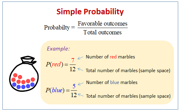
Example 1: Simple Example

A player takes 10 penalty shots and scores 6 goals.
P(Goal)=610=0.6P(\text{Goal}) = \frac{6}{10} = 0.6P(Goal)=106=0.6
👉 Probability of scoring = 0.6 or 60%

Example 2: Toss in Sports

A coin is tossed before a match.
- Total outcomes = 2 (Head, Tail)
  Probability of Head = 1/2 = 0.5

Types of Events

Certain Event → P = 1 (Sun rises every day)
Impossible Event → P = 0
Random Event → P between 0 and 1 (winning a match)

c) BINOMIAL DISTRIBUTION

Meaning

The binomial distribution is a probability distribution that deals with events having only two possible outcomes:

Success / Failure
Yes / No
Win / Lose
Goal / No Goal

Conditions of Binomial Distribution

Fixed number of trials
Each trial has two outcomes.
The probability of success remains constant.
Trials are independent

Formula (For Exam)

Example (Physical Education)

A basketball player has a 70% chance of scoring a free throw.
He attempts 5 shots.
The probability of scoring exactly 3 shots can be calculated using the Binomial Distribution.
Used to predict performance.

d) RELATION WITH NORMAL DISTRIBUTION

Connection

When the number of trials is large,
And the probability is moderate,
👉 Binomial Distribution becomes Normal Distribution

In Physical Education

Large group fitness scores
Height, weight, running time
These usually follow the Normal Distribution (bell-shaped curve).

e) RELATION WITH CORRELATION

Meaning of Correlation

Correlation shows the relationship between two variables.

Link with Probability

Probability helps in predicting outcomes
Correlation helps in measuring relationship strength.

Example

Practice time & performance
Strength & throwing distance
- 👉 Probability predicts chance,
- 👉 Correlation measuresthe relationship

🔁 SIMPLE COMPARISON

Concept	Use in PE & Sports	Example
Probability	Chance of event	Chance of winning
Binomial Distribution	Two outcomes	Goal / No Goal
Normal Distribution	Large data	Fitness scores
Correlation	Relationship	Training & performance

CONCLUSION: Probability helps predict chances, Binomial Distribution handles two-outcome events, Normal Distribution explains large performance data, and Correlation shows how sports variables are related.

Q > Normal curve: Introduction, characteristics, Skewness, Kurtosis.

🔔 NORMAL CURVE (Normal Distribution Curve)

a) INTRODUCTION

Meaning

The Normal Curve is a bell-shaped curve that represents the Normal Distribution of data.
Most values lie near the average (mean), and fewer values lie at the extremes.

In Simple Words

Most students perform average level
Few perform very well or very poorly.

Example (Physical Education)

If we plot the 100 m running times of a large group of students, the graph usually forms a bell shape, called the Normal Curve.

RELATION WITH NORMAL DISTRIBUTION

The normal curve is the graphical form of Normal Distribution
Normal Distribution describes data mathematically.
The normal curve shows it visually.

b) CHARACTERISTICS OF A NORMAL CURVE

Bell-shaped and symmetrical
Mean = Median = Mode
The highest point is at the centre.
The curve is symmetrical on both sides.
Total area under curve = 1 (100%)
The curve never touches the X-axis.s
Most values lie near the mean.
Shape is smooth and continuous.
An equal number of observations on both sides
Common in biological & sports data

Example in PE: Height, weight, reaction time, endurance, intelligence, and fitness scores usually follow a normal curve.

c) SKEWNESS

Meaning

Skewness shows the degree of asymmetry (lack of symmetry) in a distribution.

👉 Types of Skewness

✅ i) Positive Skewness

The tail is longer on the right side
Mean > Median > Mode
Example: Most students score low marks, a few score very high in a fitness test.

✅ ii) Negative Skewness

The tail is longer on the left side.
Mean < Median < Mode
Example: Most students perform well, few perform poorly.

✅ iii) Zero Skewness

Perfectly symmetrical
Mean = Median = Mode
Example: Ideal normal distribution of height.

d) KURTOSIS

Meaning

Kurtosis shows the peakedness or flatness of a curve compared to a normal curve.

👉 Types of Kurtosis

✅ i) Mesokurtic

Normal peak
Ideal normal curve
Example: Standard fitness scores.

✅ ii) Leptokurtic

High and narrow peak
Data are closely clustered.
Example: Elite athletes with similar performance.

✅ iii) Platykurtic

Flat and wide peak
Data are widely spread.d
Example: Mixed-ability students in a class.

🔗 RELATION WITH CORRELATION

Connection
- Normal distribution helps in accurate correlation analysis
- Pearson’s correlation works best when the data is normally distributed.
Example
- Height & weight
- Practice hours & performance
👉 When data follows a normal curve, correlation results are more reliable.

e) SIMPLE SUMMARY TABLE

Concept	Meaning	PE Example
Normal Curve	Bell-shaped graph	Fitness scores
Skewness	Symmetry of data	Performance levels
Kurtosis	Peak of the curve	Player consistency
Correlation	Relationship between variables	Training & results

CONCLUSION: The Normal Curve explains how most physical and sports performances are distributed, while skewness and kurtosis describe its shape, and correlation measures relationships within normally distributed data.

Q > Correlation: Meaning, type, merits.

a) MEANING OF CORRELATION

Correlation means the relationship between two variables.
It tells us how changes in one variable are related to changes in another.
- If one variable increases and the other also increases → positive relationship
- If one increases and the other decreases → negative relationship
- If no relationship exists → zero correlation

Simple Example (PE)

Practice time and performance
Height and weight
Strength and throwing distance

Correlation helps us understand how strongly these variables are connected.

b) TYPES OF CORRELATION

✅ i) Positive Correlation

When both variables increase or decrease together.
Example:
- More practice → better performance
- Taller players → greater reach

✅ ii) Negative Correlation

When one variable increases and the other decreases.
Example:
- More fatigue → less performance
- Increase in body fat → decrease in speed

✅ iii) Zero (No) Correlation

When no relationship exists between variables.
Example:
- Shoe color and running speed
- Jersey number and fitness level

✅ iv) Perfect Correlation

Perfect Positive: r = +1
Perfect Negative: r = −1
Example: Exact increase of training days and fitness score (ideal case)

c) MERITS (ADVANTAGES) OF CORRELATION

Shows the relationship between variables
Helps in the prediction of performance
Useful in sports research
Assists in training planning
Helps coaches in decision-making
Useful for talent identification
Saves time and effort
Helps in performance evaluation
Supports scientific approach in PE
Makes data analysis easy and meaningful

d) RELATION WITH NORMAL DISTRIBUTION

Connection Explained Simply

Correlation works best when data follows a Normal Distribution
Pearson’s correlation coefficient assumes:
- Data is normally distributed.
- The relationship is linear.
Example: The height and weight of students usually follow a normal curve, So the correlation between them is accurate and reliable.

CORRELATION & NORMAL CURVE – LINK

Concept	Role
Normal Distribution	Shows how data is spread
Normal Curve	Graphical form of distribution
Correlation	Measures the relationship between variables

👉 Normally distributed data gives better correlation results.

CONCLUSION: Correlation helps Physical Education teachers and coaches understand how different physical and performance variables are related, especially when data follows a normal distribution.

Q > Product-moment correlation, Rank order method

CORRELATION (Methods)

Correlation helps us know how strongly two variables are related, such as training and performance or height and weight.

a) PRODUCT–MOMENT CORRELATION

(Karl Pearson’s Coefficient of Correlation)

Meaning
- Product-Moment Correlation measures the degree and direction of the relationship between two continuous variables.
- It is the most commonly used correlation method.
Symbol = r
Value of r
- r = +1 → Perfect positive correlation
- r = −1 → Perfect negative correlation
- r = 0 → No correlation
Formula (For Exams)
- r=Σ(x−xˉ)(y−yˉ)Σ(x−xˉ)2Σ(y−yˉ)2r = \frac{Σ(x – \bar{x})(y – \bar{y})}{\sqrt{Σ(x – \bar{x})^2 Σ(y – \bar{y})^2}}r=Σ(x−xˉ)2Σ(y−yˉ)2Σ(x−xˉ)(y−yˉ)
Example (Physical Education)
- Variables:
  - Practice hours
  - Performance score
- If students who practice more score higher, the correlation will be positive.
- Example conclusion:
  - r = +0.75 → High positive correlation
When to Use
- Data is quantitative (numerical)
- The relationship is linear.
- Data is normally distributed.
Importance in PE
- Used in sports science research
- Helps predict future performance
- Useful in fitness testing analysis

b) RANK ORDER METHOD

(Spearman’s Rank Correlation)

Meaning
- Rank Order Method measures the relationship between ranks, not actual scores.
- It is used when data is in rank form.
Symbol = ρ (rho)
Formula
- ρ=1−6Σd2n(n2−1)ρ = 1 – \frac{6Σd^2}{n(n^2 – 1)}ρ=1−n(n2−1)6Σd2
- Where:
  - d = difference between ranks
  - n = number of pairs
Example (Physical Education)
- Ranks in fitness test and sports performance:
- Small rank differences → high correlation

Student	Fitness Rank	Performance Rank
A	1	2
B	2	1
C	3	3

When to Use
- Data is in ranks
- The distribution is not normal.
- The sample size is small.l
Importance in PE
- Used in talent selection
- Useful when scores are unavailable
- Easy to calculate and understand

c) RELATION WITH NORMAL DISTRIBUTION

Connection Explained Simply

Method	Relation with Normal Distribution
Product-Moment	Assumes normal distribution
Rank Order	Does not require normal distribution

👉 Normally distributed data → Product-Moment is best
👉 Non-normal or ranked data → Rank Order is best

🔁 COMPARISON TABLE

Point	Product-Moment (Karl Pearson)	Rank Order (Spearman)
Data Type	Continuous	Rank data
Symbol	r	ρ
Normal Distribution	Required	Not required
Accuracy	High	Moderate
Use in PE	Research studies	Talent ranking

CONCLUSION: Product-Moment Correlation is best for normally distributed numerical data, while Rank Order Correlation is suitable for ranked or non-normal data in Physical Education.

Unit 4:- Significance of Test

Q > Small sample: Introduction, Student t distribution,

a) SMALL SAMPLE – INTRODUCTION

Meaning
- A small sample is a group of observations with a small size, usually less than 30 (n < 30).
- In Physical Education research, we often work with small samples due to limited players or students.
Why Small Samples are Used
- Difficult to get large groups of athletes
- Time and cost limitations
- Experimental training programs
- Case studies and pilot studies
Example (Physical Education)
- A coach studies the effect of 4-week plyometric training on 12 athletes.
- Here, 12 athletes = small sample.
Problem with Small Samples
- Results may vary more
- The normal distribution assumption may not be reliable.
- So, special statistical methods are needed

b) STUDENT’S t-DISTRIBUTION

Meaning
Student’s t-distribution is a probability distribution used when:
- Sample size is small (n < 30)
- The population standard deviation is unknown.n
- Data is approximately normally distributed.
It was developed by William Sealy Gosset, who used the name “Student”.
Shape of t-Distribution
- Similar to a normal curve
- More spread out (wider tails)
- Becomes normal distribution as the sample size increases

Types of t-Tests (For PE Exams)

✅ i) One-sample t-test
- Compare the sample mean with a known value
- Example: Average stamina score vs standard norm
✅ ii) Independent t-test
- Compare two different groups.
- Example: Boys vs girls fitness scores
✅ iii) Paired t-test
- Compare before and after training.
- Example: Performance before & after training

Simple Formula
- t=xˉ−μs/nt = \frac{\bar{x} – \mu}{s/\sqrt{n}}t=s/nxˉ−μ
- Where:
  - x̄ = sample mean
  - μ = population mean
  - s = sample standard deviation
  - n = sample size

c) RELATION WITH SIGNIFICANCE OF TEST

Meaning of Significance: A significant test tells us whether the result is real or due to chance.
How the t-Test Shows Significance
- The calculated t value is compared with the table value.
- If calculated t > table t 👉 Result is significant
- If calculated t < table t 👉 Result is not significant
Example (PE)
- After a training program:
- Calculated t = 2.5
- Table t (0.05 level) = 2.18
  - 👉 2.5 > 2.18
  - 👉 The training program is significant

🔄 LINK WITH NORMAL DISTRIBUTION

Small Sample	Large Sample
Uses t-distribution	Uses normal distribution
n < 30	n ≥ 30
Population SD unknown	Population SD known

👉 As the sample size increases, the t-distribution becomes a normal distribution.

CONCLUSION: In Physical Education research, small samples require Student’s t-distribution to test the significance of results and ensure that improvements are not due to chance.

Q > Student t-test (Independent)

a) INTRODUCTION / MEANING

The Independent t-test is used to compare the means (averages) of two separate and unrelated groups to determine whether the difference between them is real or due to chance.
The two groups must be independent, meaning no subject is common to both groups.

🔹 WHEN DO WE USE THE INDEPENDENT t-TEST?

We use the Independent t-test when:

Sample size is small (n < 30)
Two different groups are compared.
Data is quantitative
The population standard deviation is unknown.n
Data is approximately normally distributed.

🔹 EXAMPLES IN PHYSICAL EDUCATION

Boys vs Girls’ physical fitness scores
Trained vs Untrained Athletes
Urban vs Rural students’ endurance levels
Team A vs Team B performance scores

🔹 ASSUMPTIONS (Simple)

Groups are independent
Data is normally distributed.
The variance of both groups is approximately equal.

b) FORMULA (For Exam)

t=Xˉ1−Xˉ2S12n1+S22n2t = \frac{\bar{X}_1 – \bar{X}_2}{\sqrt{\frac{S_1^2}{n_1} + \frac{S_2^2}{n_2}}}t=n1S12+n2S22Xˉ1−Xˉ2

Where:

Xˉ1,Xˉ2\bar{X}_1, \bar{X}_2Xˉ1,Xˉ2 = Means of two groups
S1,S2S_1, S_2S1,S2 = Standard deviations
n1,n2n_1, n_2n1,n2 = Sample sizes

🔹 STEP-BY-STEP PROCEDURE (Very Simple)

Find the mean of both groups
Find the standard deviation of both groups.
Substitute values in the formula
Calculate t-value
Compare with the table value of t

c) SIGNIFICANCE OF THE TEST

✅ What is Significance?

Significance tells us whether the difference between two group means is genuine or happened by chance.

✅ Decision Rule

Condition	Result
Calculated t > Table t	Significant difference
Calculated t < Table t	Not significant

✅ SIMPLE EXAMPLE (PE-Based)

Fitness scores of two groups:

Group	Mean Score	n
Boys	55	12
Girls	48	12

Calculated t = 2.6
Table t at 0.05 level = 2.18
- 👉 Since 2.6 > 2.18,
- 👉 Difference is statistically significant

Conclusion: Boys performed better than girls in the fitness test.

✅ LEVELS OF SIGNIFICANCE

0.05 level → 95% confidence
0.01 level → 99% confidence

Lower value = stricter test

CONCLUSION: The Independent Student t-test helps Physical Education teachers and researchers determine whether the difference between two separate groups is statistically significant or just due to chance.

Q > Paired T-Test (dependent)

a) Meaning of Paired T-Test

The Paired t-test is used to compare the means of the same group measured at two different times or under two different conditions.
The data are called dependent because each score in the first test is paired with a related score in the second test.
It checks whether the change in performance is real or due to chance.

🔹 WHEN DO WE USE A PAIRED t-TEST?

We use the Paired t-test when:

The same subjects are tested twice
Sample size is small (n < 30)
Data is quantitative
The population standard deviation is unknown.
Data is approximately normally distributed.

🔹 EXAMPLES IN PHYSICAL EDUCATION

Fitness test before and after training
Skill performance pre-test and post-test
Endurance level before and after conditioning
Flexibility test before and after yoga practice

🔹 SIMPLE ASSUMPTIONS

Same participants in both tests
Difference scores are normally distributed.
Observations are related (paired)

b) FORMULA (FOR EXAM)

t=dˉsd/nt = \frac{\bar{d}}{s_d / \sqrt{n}}t=sd/ndˉ

Where:

dˉ\bar{d}dˉ = Mean of differences
sds_dsd = Standard deviation of differences
nnn = Number of pairs

🔹 STEP-BY-STEP PROCEDURE (EASY)

Find the difference (d) between pre-test and post-test scores
Calculate the mean of differences (d̄)
Calculate the standard deviation of differences.
Substitute values in the formula
Find the calculated t-value
Compare with the table t-value

c) SIGNIFICANCE OF THE TEST

🔹What is Significance?

Significance indicates whether the improvement or decline is real or has occurred by chance.

DECISION RULE

Condition	Result
Calculated t > Table t	Significant difference
Calculated t < Table t	Not significant

🔹 SIMPLE PE EXAMPLE

Endurance scores of 10 students:

Test	Mean Score
Before Training	42
After Training	50

Calculated t = 3.1
Table t at 0.05 level = 2.26
- Since 3.1 > 2.26,
- Improvement is statistically significant

Conclusion: The training program effectively improved endurance.

🔹 DEGREE OF FREEDOM

df=n−1df = n – 1df=n−1

CONCLUSION: The Paired t-test helps Physical Education teachers and researchers determine whether changes in performance within the same group are statistically significant.

Q > Large sample: Z- test

a) Meaning of Z- test

The Z-test is a statistical test used to compare averages (means) when the sample size is large.
A large sample generally means 30 or more observations (n ≥ 30).
The Z-test helps us decide whether the difference between means is real or occurred by chance.

🔹 WHEN DO WE USE Z-TEST?

We use the Z-test when:

Sample size is large (n ≥ 30)
Data is quantitative (numerical)
Population standard deviation is known, or the sample size is large.
Data is approximately normally distributed.

🔹 TYPES OF Z-TEST (Simple)

One-sample Z-test – Compare sample mean with a known population mean
Two-sample Z-test – Compare means of two large independent groups

🔹 EXAMPLES IN PHYSICAL EDUCATION

Comparing the average fitness score of 100 students with a standard norm
Comparing the performance of two large groups (e.g., 60 boys vs 60 girls)
Checking the effectiveness of a training program on a large group of athletes

b) FORMULA (FOR EXAM)

✅ i) One-Sample Z-Test

Z=Xˉ−μσ/nZ = \frac{\bar{X} – \mu}{\sigma / \sqrt{n}}Z=σ/nXˉ−μ

✅ ii) Two-Sample Z-Test

Z=Xˉ1−Xˉ2σ12n1+σ22n2Z = \frac{\bar{X}_1 – \bar{X}_2}{\sqrt{\frac{\sigma_1^2}{n_1} + \frac{\sigma_2^2}{n_2}}}Z=n1σ12+n2σ22Xˉ1−Xˉ2

Where:

Xˉ\bar{X}Xˉ = Sample mean
μ\muμ = Population mean
σ\sigmaσ = Population standard deviation
nnn = Sample size

🔹 STEP-BY-STEP PROCEDURE (EASY)

State null hypothesis (H₀)
Choose the level of significance (0.05 or 0.01)
Calculate the Z-value using the formula.
Compare with the table Z-value.
Draw conclusion

c) SIGNIFICANCE OF THE TEST

Meaning: Significance tells us whether the difference observed is genuine or due to chance.

DECISION RULE

Level of Significance	Table Z-Value
0.05 level	±1.96
0.01 level	±2.58

Condition	Decision
Calculated Z > Table Z	Significant
Calculated Z < Table Z	Not Significant

🔹 SIMPLE PE EXAMPLE

A fitness norm says the average endurance score should be 50.
From a sample of 60 students:
- Mean score = 53
- SD = 6
Calculated Z = 2.2
Table Z (0.05) = 1.96
- Since 2.2 > 1.96,
- The result is statistically significant

Conclusion: Students’ endurance is better than the norm.

🔹 RELATION WITH NORMAL DISTRIBUTION

The Z-test is based on the Normal Distribution
Z-scores measure how far a value is from the mean in standard units.
Large samples follow the normal curve due to the Central Limit Theorem.

📌 CONCLUSION

The Z-test is used in Physical Education research to test the significance of results when the sample size is large and the data follow a normal distribution.